Learning how to learn

Author: Rui

From Keywords to Context: What AI’s Intent Understanding Means for Content Creators
The shift from keyword matching to contextual understanding means content creators must write for comprehension, not just discovery. AI systems don’t just match words—they understand intent, context, and the unstated needs behind every query.

In my first post, I explored how both traditional and AI-powered search follow the same fundamental steps: crawl and index content, understand user intent, then match and retrieve content. This sequence hasn’t changed. What has changed is now AI-powered search embeds Large Language Models (LLMs) into each step.

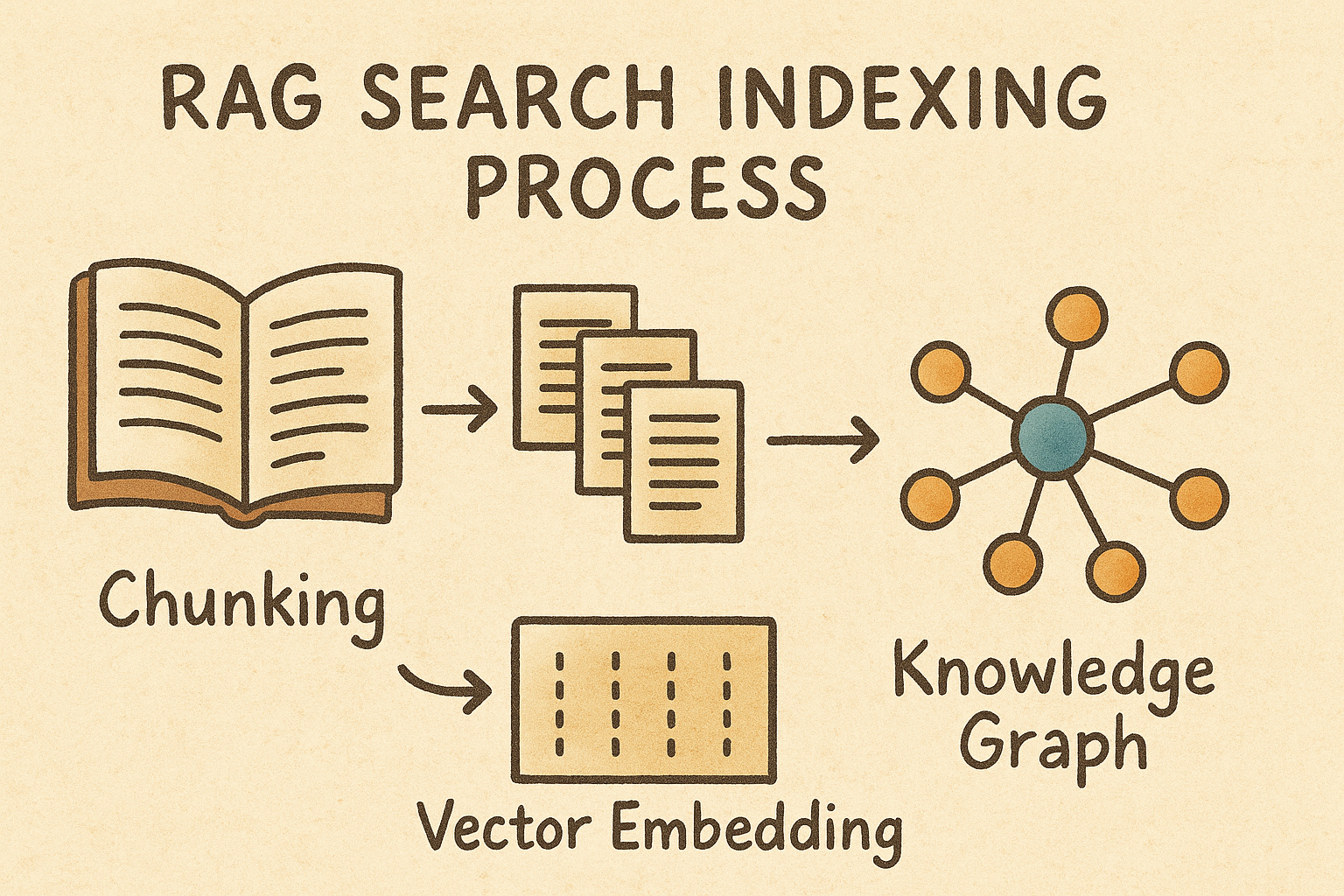
My last post dove deep into indexing step, explaining how AI systems use vector embeddings and knowledge graphs to chunk content semantically. AI systems understand meaning and relationships rather than cataloging keywords.

So what’s different about user query (intent) understanding? When someone searches for “How to make my computer faster?“, what are they really asking for?

Traditional search engines and AI-powered search systems interpret this question in fundamentally different ways. , with profound implications for how we should create content.

The Evolution of Intent Understanding

To appreciate how revolutionary AI-driven intent understanding is, we need to look at how search has evolved.

The evolution of search intent understanding

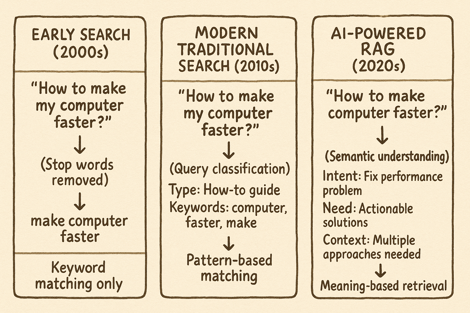
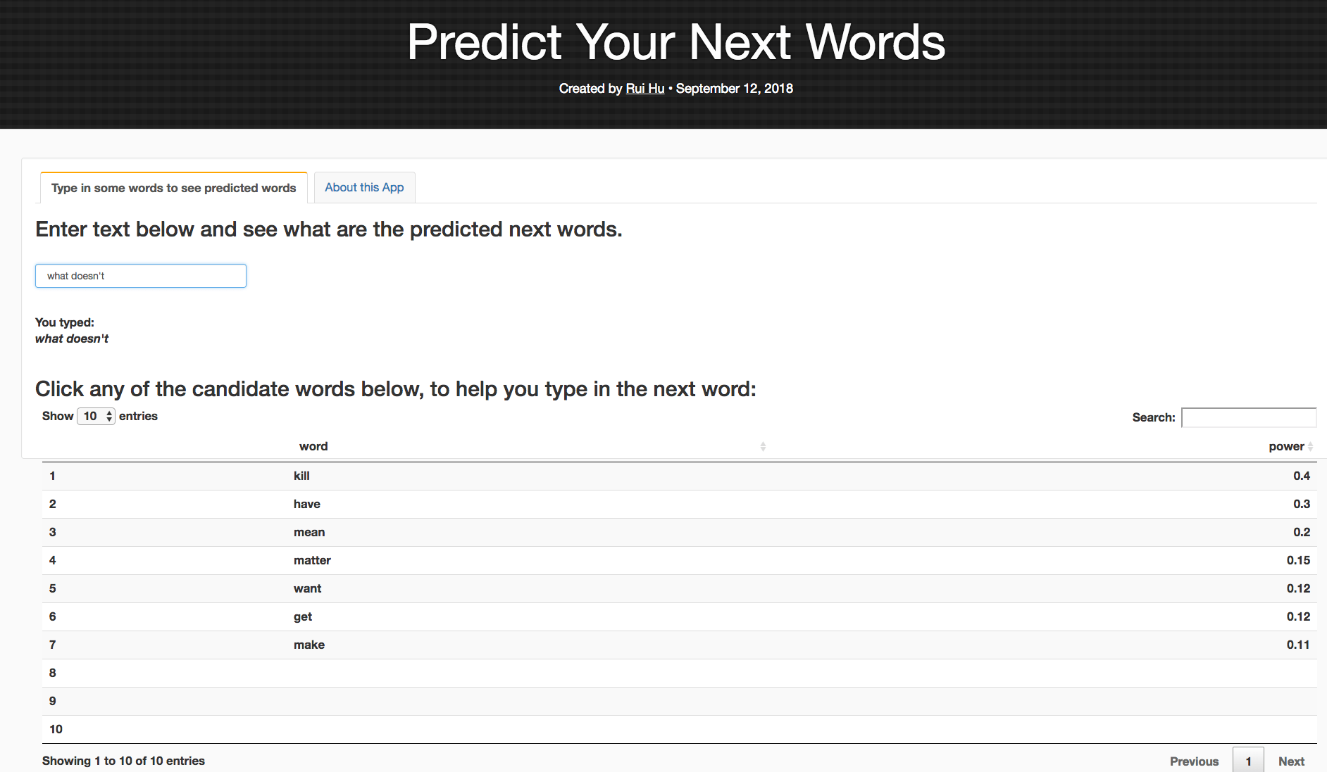
Early traditional search engines treated question words like “how,” “why,” and “where” as “stop words”—filtering them out before processing queries.

Modern traditional search has evolved to preserve question words and use them for basic query classification. But the understanding remains relatively shallow—more like categorization than true comprehension.

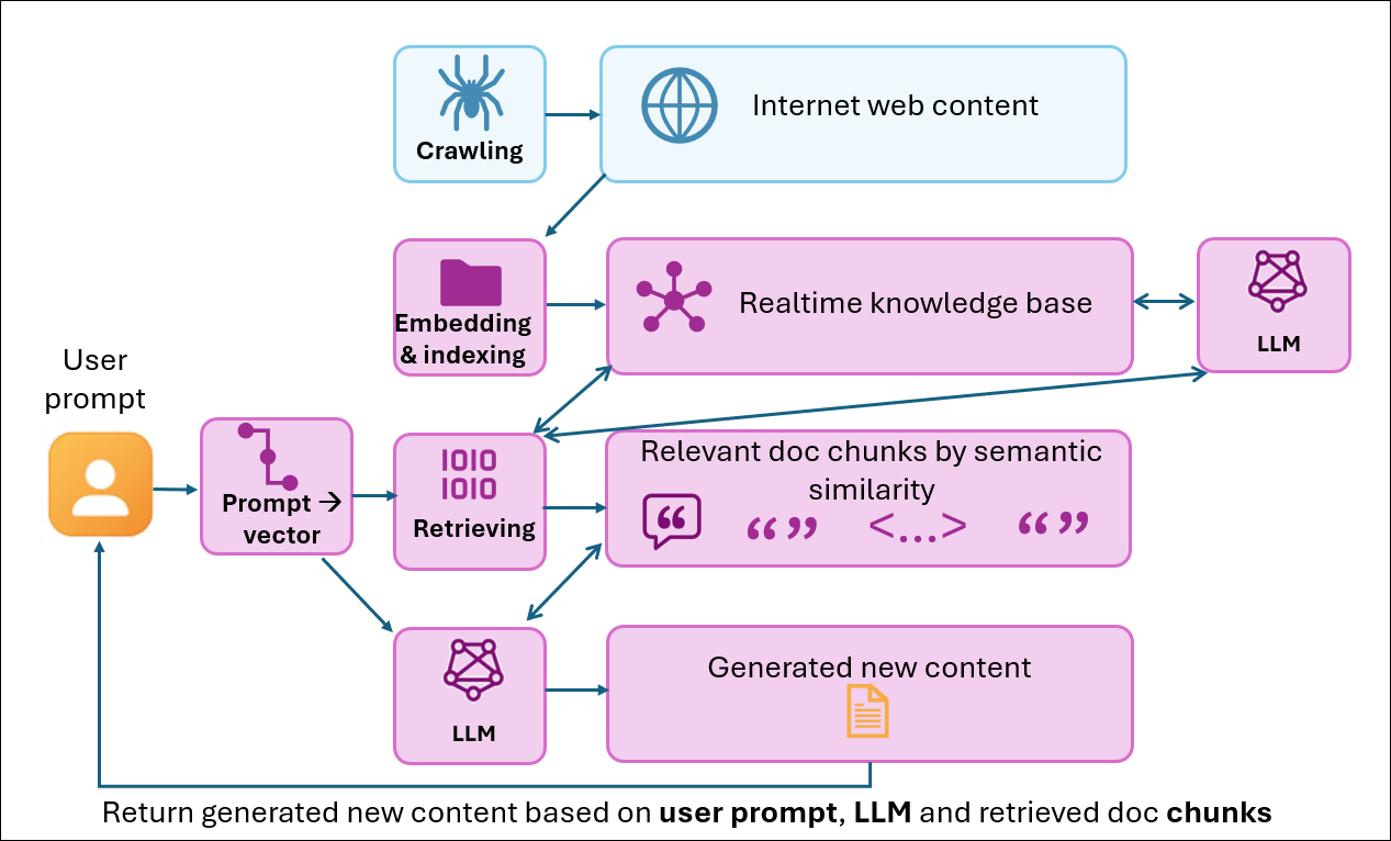
AI-powered RAG (Retrieval-Augmented Generation) systems represent a fundamental leap. They decode the full semantic meaning, understand user context, and map queries to solution pathways.

Modern Traditional Search: Pattern Recognition

Let’s examine how modern traditional search processes our example query “How to make my computer faster?”

Traditional search recognizes that “How to” signals an instructional query and knows that “computer faster” relates to performance. Yet it treats these as isolated signals rather than understanding the complete situation.

Traditional search processes the query through tokenization, preserving “How to” as a query classifier while removing low-value words like “my.” It then applies pattern recognition to classify the query type as instructional and identifies keywords related to computer performance optimization.

What it can’t understand:
- "My” implies the user has an actual problem right now—not theoretical interest
- “Make...faster” suggests current dissatisfaction requiring immediate solutions
- The question format expects comprehensive guidance, not scattered tips
- A performance problem likely has multiple causes needing different approaches
AI Search: Deep Semantic Comprehension

RAG systems process the same query through multiple layers of understanding:

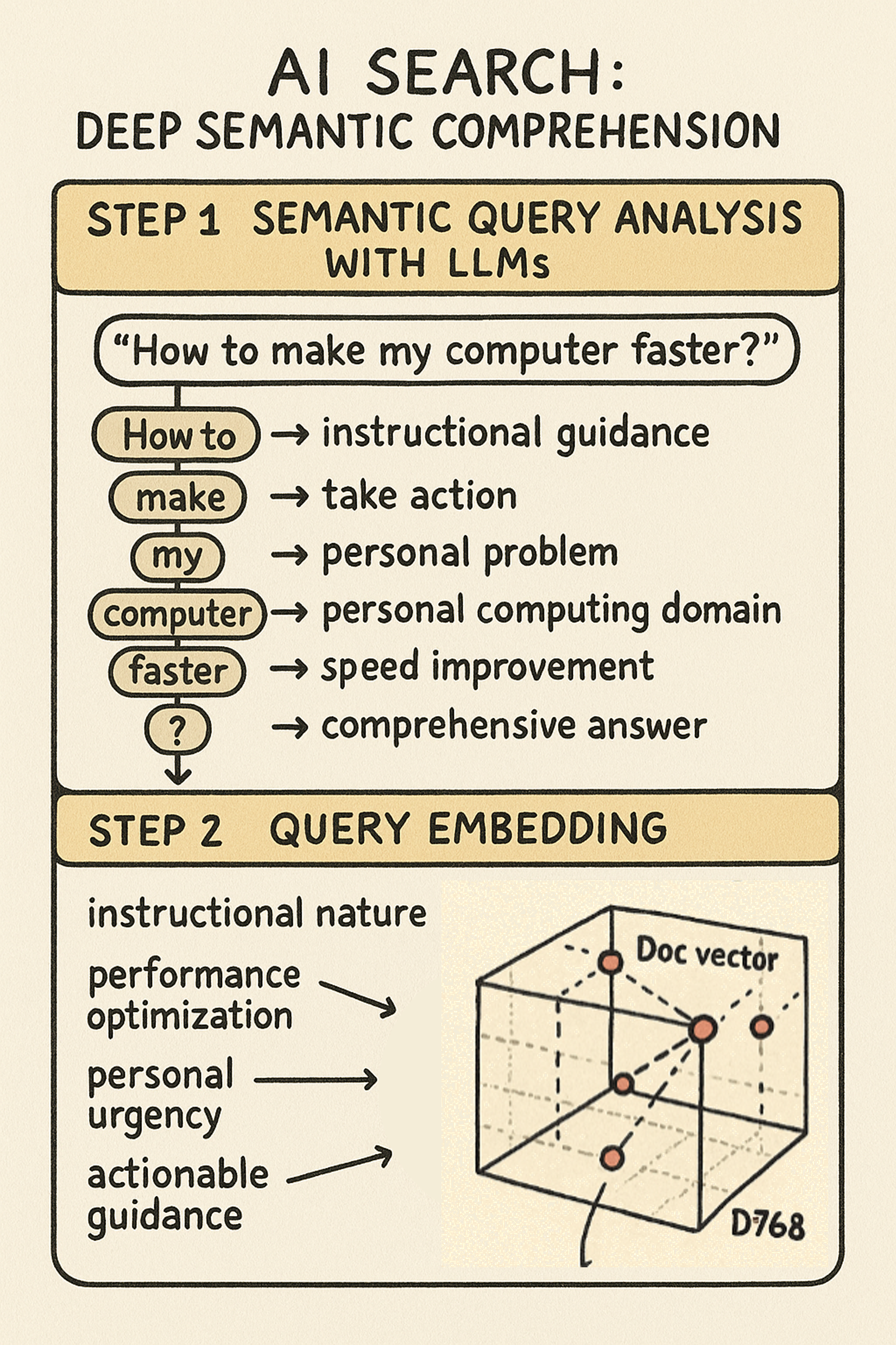
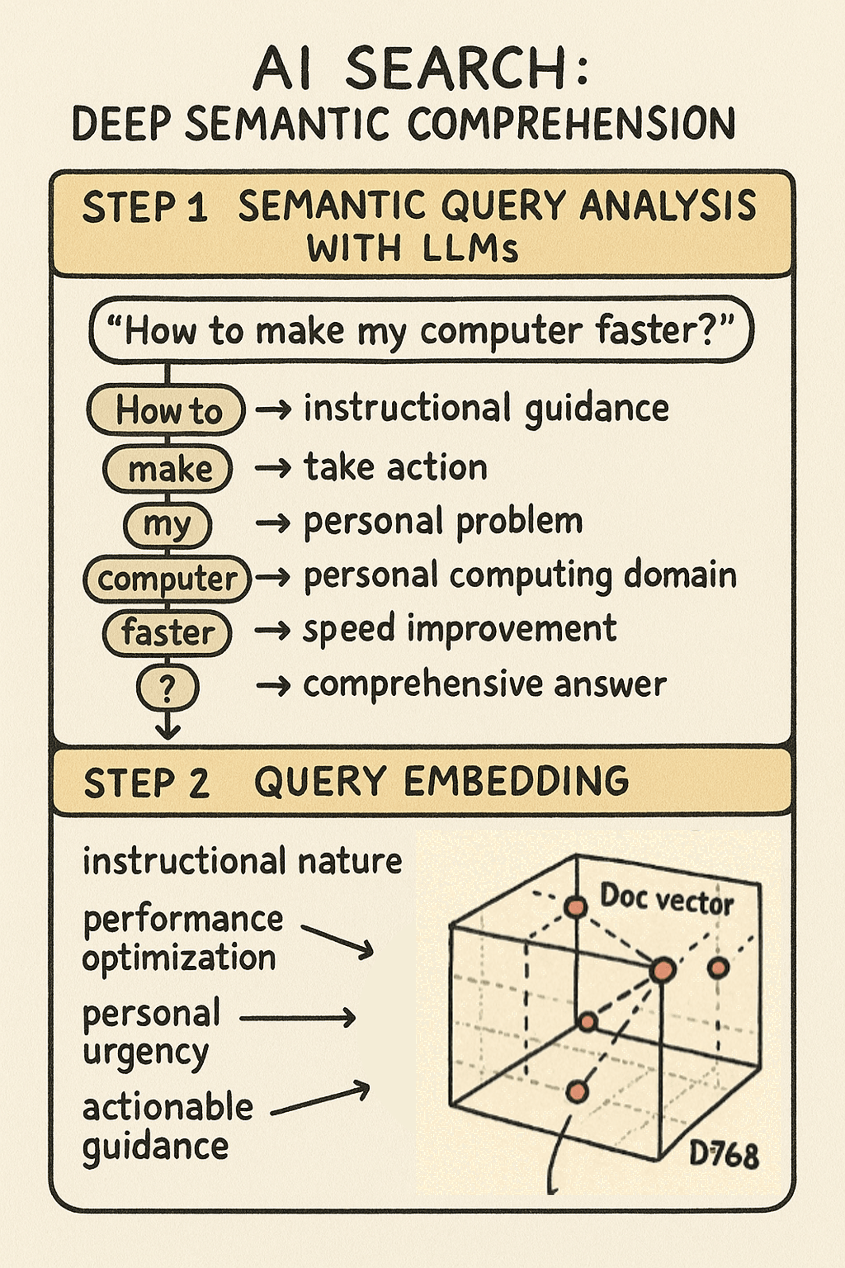
Semantic Query Analysis When the AI receives “How to make my computer faster?”, it decodes the question’s semantic meaning:
- “How to“ → User needs instructional guidance, not just information
- “make“ → User wants to take action, transform current state
- “my“ → Personal problem happening now, not hypothetical
- “computer“ → Specific domain: personal computing, not servers or networks
- “faster“ → Performance dissatisfaction, seeking speed improvement
- “?“ → Expects comprehensive answer, not yes/no response
The LLM understands this isn’t someone researching computer performance theory—it’s someone frustrated with their slow computer who needs actionable solutions now.

Query Embedding The query gets converted into a vector that captures semantic meaning across hundreds of dimensions. While individual dimensions are abstract mathematical representations, the vector as a whole captures:
- The instructional nature of the request
- The performance optimization context
- The personal urgency
- The expected response type (actionable guidance)
By converting queries into the same vector space used for content indexing, AI creates the foundation for semantic matching that goes beyond keywords.

The Key Difference While traditional search sees keywords and patterns, AI comprehends the actual situation: a frustrated user with a slow computer who needs comprehensive, actionable guidance. This semantic understanding of intent becomes the foundation for retrieval and matching.

How Different Queries are Understood

This deeper understanding transforms how different queries are processed:

“Where can I find Azure pricing?“
- Traditional: Matches “Azure” + “pricing” + “find“
- RAG: Understands commercial evaluation intent, knows you’re likely comparing options
“Why is my app slow?“
- Traditional: Diagnostic query about “app” + “slow“
- RAG: Recognizes frustration, expects root-cause analysis and immediate fixes
What this Means for Content Creators

AI’s ability to understand user intent through semantic analysis and vector embeddings changes how we need to create content. Since AI understands the context behind queries (recognizing “my computer” signals a current problem needing immediate help), our content must address these deeper needs:

1. Write Like You’re Having a Conversation

Remember how AI decoded each word of “How to make my computer faster?” for semantic meaning? AI models excel at understanding natural language patterns because they’re trained on conversational data. Question-based headings (“How do I migrate my database?“) align perfectly with how users actually phrase their queries.

Instead of: “Implement authentication protocols using OAuth 2.0 framework” Write: “Here's how to set up secure login for your app using OAuth 2.0“

The conversational version provides contextual clues that help AI understand user intent:

“Here's how” signals instructional content, “your app” indicates practical guidance, and “secure login” translates technical concepts to user benefits.

2. Provide Full Context in Self-Contained Sections

AI understands that “How to make my computer faster?” requires multiple solution types—hardware, software, and maintenance. Since AI grasps these comprehensive needs through vector embeddings, your content should provide complete context within each section.

Include the why behind recommendations, when different solutions apply, and what trade-offs exist—all within the same content chunk. This aligns with how AI chunks content semantically and understands queries holistically.

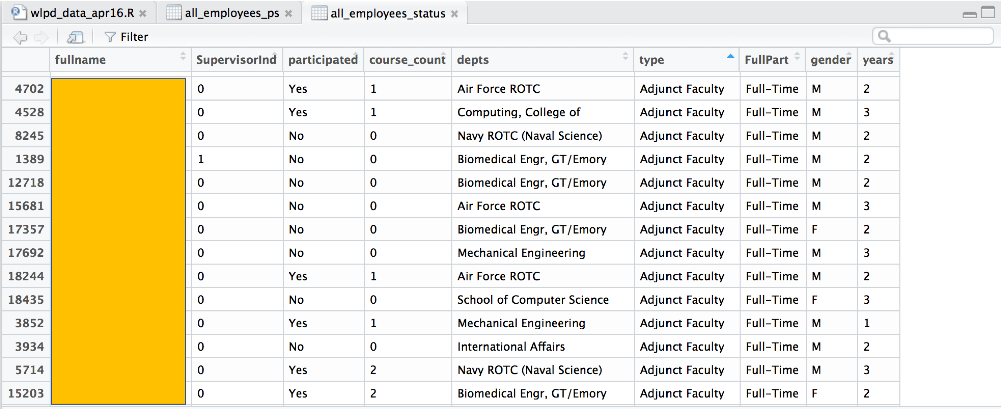
3. Use Intent-Driven Metadata

Since AI converts queries into semantic vectors that capture intent (instructional need, urgency, complexity level), providing explicit intent metadata helps AI better understand your content’s purpose:
- User intent: “As a developer, I want to implement secure authentication so that user data remains protected“
- Level: Beginner/Intermediate/Advanced to match user expertise
- Audience: Developer/Admin/End-user for role-based content alignment
This metadata becomes part of the semantic understanding, helping AI match content to the right user intent.

The Bigger Picture

AI’s semantic understanding of user intent changes content strategy fundamentals. Content creators must now focus on addressing the full context of user queries and consider the implicit needs that AI can detect.

This builds on the semantic chunking we explored in my last post. AI systems use the same vector embedding approach for both indexing content and understanding queries. When both exist in the same semantic space, AI can connect content to user needs even when keywords don’t match.

The practical impact:

AI can now offer comprehensive, contextual answers by understanding what users need, not what they typed. But this only works when we create structured content in natural language, complete context, and clear intent signals.

This is the second post in my three-part series on AI-ready content creation. In my first post, we explored how AI indexes content through semantic chunking rather than keyword extraction.

Coming next: “Beyond Rankings: How AI Retrieval Transforms Content Discovery”

Now that we understand how AI indexes content (Post 1) and interprets user intent (this post). My next post will reveal how AI systems match and retrieve content. I’ll explore:
- How vector similarity replaces PageRank-style algorithms
- Why knowledge graphs matter more than link structures
- And what this means for making your content discoverable in AI-powered search
August 26, 2025
Understanding Indexing: A Guide for Content Creators and AI Search
In my earlier post, I explained the fundamental shift from traditional search to generative AI search. Traditional search finds existing content. Generative AI creates new responses.

If you’ve been hearing recommendations about “AI-ready content” like chunk-sized content, conversational language, Q&A formats, and structured writing, these probably sound familiar. As instructional designers and content developers, we’ve used most of these approaches for years. We chunk content for better learning, write conversationally to engage readers, and use metadata for reporting and semantic web purposes.

Today, I want to examine how this shift starts at the very beginning: when systems index and process content.

What is Indexing?

Indexing is how search systems break down and organize content to make it searchable. Traditional search creates keyword indexes, while AI search creates vector embeddings and knowledge graphs from semantic chunks. The move from keywords to chunks signifies one of the most significant changes in how search technology works.

Let’s trace how both systems process the same content using three sample documents from my previous post:

Document 1: “Upgrading your computer's hard drive to a solid-state drive (SSD) can dramatically improve performance. SSDs provide faster boot times and quicker file access compared to traditional drives.“

Document 2: “Slow computer performance is often caused by too many programs running simultaneously. Close unnecessary background programs and disable startup applications to fix speed issues.“

Document 3: “Regular computer maintenance prevents performance problems. Clean temporary files, update software, and run system diagnostics to keep your computer running efficiently.“

User query: “How to make my computer faster?“

How does traditional search index content?

Traditional search follows three mechanical steps:

Step 1: Tokenization

This step breaks raw text into individual words. The three docs after tokenization look like this:
```
DOC1 → Tokenization → ["Upgrading", "your", "computer's", "hard", "drive", "to", "a", "solid-state", "drive", "SSD", "can", "dramatically", "improve", "performance", "SSDs", "provide", "faster", "boot", "times", "and", "quicker", "file", "access", "compared", "to", "traditional", "drives"]

DOC2 → Tokenization → ["Slow", "computer", "performance", "is", "often", "caused", "by", "too", "many", "programs", "running", "simultaneously", "Close", "unnecessary", "background", "programs", "and", "disable", "startup", "applications", "to", "fix", "speed", "issues"]

DOC3 → Tokenization → ["Regular", "computer", "maintenance", "prevents", "performance", "problems", "Clean", "temporary", "files", "update", "software", "and", "run", "system", "diagnostics", "to", "keep", "your", "computer", "running", "efficiently"]
```
Step 2: Stop Word Removal & Stemming

What are Stop Words?

Stop words are common words that appear frequently in text but carry little meaningful information for search purposes. They’re typically removed during text preprocessing to focus on content-bearing words.

Common English stop words:
```
a, an, the, is, are, was, were, be, been, being, have, has, had, do, does, did, will, would, could, should, may, might, can, of, in, on, at, by, for, with, to, from, up, down, into, over, under, and, or, but, not, no, yes, this, that, these, those, here, there, when, where, why, how, what, who, which, your, my, our, their
```
What is Stemming?

Stemming is the process of reducing words to their root form by removing suffixes, prefixes, and other word endings. The goal is to treat different forms of the same word as identical for search purposes.

Some stemming Examples:
```
Original Word    →    Stemmed Form
"running"        →    "run"
"runs"           →    "run"  
"runner"         →    "run"
"performance"    →    "perform"
"performed"      →    "perform"
"performing"     →    "perform"
```
The three sample documents after stop words removal and stemming look like this:
```
DOC1 Terms: ["upgrad", "comput", "hard", "driv", "solid", "stat", "ssd", "dramat", "improv", "perform", "ssd", "provid", "fast", "boot", "time", "quick", "file", "access", "compar", "tradit", "driv"]

DOC2 Terms: ["slow", "comput", "perform", "caus", "program", "run", "simultan", "clos", "unnecessari", "background", "program", "disabl", "startup", "applic", "fix", "speed", "issu"]

DOC3 Terms: ["regular", "comput", "maintain", "prevent", "perform", "problem", "clean", "temporari", "file", "updat", "softwar", "run", "system", "diagnost", "keep", "comput", "run", "effici"]
```
Step 3: Inverted Index Construction

What is inverted index?

An inverted index is like a book’s index, but instead of mapping topics to page numbers, it maps each unique word to all the documents that contain it. It’s called “inverted” because instead of going from documents to words, it goes from words to documents.
Note: For clarity and space, I’m showing only a representative subset that demonstrates key patterns.

The complete inverted index would contain entries for all ~28 unique terms from our processed documents. The key patterns include:
- Terms appearing in all documents (common terms like “comput”)
- Terms unique to one document (distinctive terms like “ssd”)
- Terms with varying frequencies (like “program” with tf=2)
```
INVERTED INDEX:
"comput" → {DOC1: tf=1, DOC2: tf=1, DOC3: tf=1}
"perform" → {DOC1: tf=1, DOC2: tf=1, DOC3: tf=1}
"fast" → {DOC1: tf=1}
"speed" → {DOC2: tf=1}
"ssd" → {DOC1: tf=1}
"program" → {DOC2: tf=2}
"maintain" → {DOC3: tf=1}
"slow" → {DOC2: tf=1}
"improv" → {DOC1: tf=1}
"fix" → {DOC2: tf=1}
"clean" → {DOC3: tf=1}
```
The result: An inverted index that maps each word to the documents containing it, along with frequency counts.

Why inverted indexing matters for content creators:

Traditional search relies on keyword matching. This is why SEO focused on keyword density and exact phrase matching.

How do AI systems index content?

AI systems take a fundamentally different approach:

Step 1: Semantic chunking

AI doesn’t break content into words. Instead, it creates meaningful, self-contained chunks. AI systems analyze content for topic boundaries, logical sections, and complete thoughts to determine where to split content. They look for natural break points that preserve context and meaning.

What AI Systems Look For When Chunking

1. Semantic Coherence
- Topic consistency: Does this section maintain the same subject matter?
- Conceptual relationships: Are these sentences talking about related ideas?
- Context dependency: Do these sentences need each other to make sense?
2. Structural Signals
- HTML tags: Headings (H1, H2, H3), paragraphs, lists, sections
- Formatting cues: Line breaks, bullet points, numbered steps
- Visual hierarchy: How content is organized on the page
3. Linguistic Patterns
- Transition words: “However,” “Therefore,” “Next,” “Additionally”
- Pronoun references: “It,” “This,” “These” that refer to previous concepts
- Discourse markers: Words that signal topic shifts or continuations
4. Completeness of Information
- Self-contained units: Can this chunk answer a question independently?
- Context sufficiency: Does the chunk have enough background to be understood?
- Action completeness: For instructions, does it contain a complete process?
5. Optimal Size Constraints
- Token limits: Most AI models have processing windows (512, 1024, 4096 tokens)
- Embedding efficiency: Chunks need to be small enough for accurate vector representation
- Memory constraints: Balance between context preservation and processing speed
6. Content Type Recognition
- Question-answer pairs: Natural chunk boundaries
- Step-by-step instructions: Each step or related steps become chunks
- Examples and explanations: Keep examples with their explanations
- Lists and enumerations: Group related list items
For demonstration purposes, I’m breaking our sample documents by sentences, though real AI systems use more sophisticated semantic analysis:
```
DOC1 → Chunk 1A: "Upgrading your computer's hard drive to a solid-state drive (SSD) can dramatically improve performance."
DOC1 → Chunk 1B: "SSDs provide faster boot times and quicker file access compared to traditional drives."

DOC2 → Chunk 2A: "Slow computer performance is often caused by too many programs running simultaneously."
DOC2 → Chunk 2B: "Close unnecessary background programs and disable startup applications to fix speed issues."

DOC3 → Chunk 3A: "Regular computer maintenance prevents performance problems."
DOC3 → Chunk 3B: "Clean temporary files, update software, and run system diagnostics to keep your computer running efficiently."
```
Step 2: Vector embedding

Vector embeddings are created using pre-trained transformer neural networks like BERT, RoBERTa, or Sentence-BERT. These models have already learned semantic relationships from massive text datasets. Chunks are tokenized first, then passed through the pre-trained models. After that, each chunk becomes a mathematical representation of meaning.
```
Chunk 1A → Embedding: [0.23, -0.45, 0.78, ..., 0.67] (768 dims)
    Semantic Concepts: Hardware upgrade, SSD technology, performance improvement
    
Chunk 1B → Embedding: [0.18, -0.32, 0.81, ..., 0.71] (768 dims)  
    Semantic Concepts: Speed benefits, boot performance, storage comparison
    
Chunk 2A → Embedding: [-0.12, 0.67, 0.34, ..., 0.23] (768 dims)
    Semantic Concepts: Performance issues, software conflicts, resource problems
    
Chunk 2B → Embedding: [-0.08, 0.71, 0.29, ..., 0.31] (768 dims)
    Semantic Concepts: Software optimization, process management, troubleshooting
    
Chunk 3A → Embedding: [0.45, 0.12, -0.23, ..., 0.56] (768 dims)
    Semantic Concepts: Preventive care, maintenance philosophy, problem prevention
    
Chunk 3B → Embedding: [0.41, 0.18, -0.19, ..., 0.61] (768 dims)
    Semantic Concepts: Maintenance tasks, system care, routine optimization
```
Step 3: Knowledge graph construction

What is a Knowledge Graph?

Screenshot of the visualized knowledge graph based on the sample docs

A knowledge graph is a structured way to represent information as a network of connected entities and their relationships. Think of it like a map that shows how different concepts relate to each other. For example, it captures that “SSD improves performance” or “too many programs cause slowness.” This explicit relationship mapping helps AI systems understand not just what words appear together, but how concepts actually connect and influence each other.

How is knowledge graph constructed?

The system analyzes each text chunk to identify: (1) Entities – the important “things” mentioned (like Computer, SSD, Performance), (2) Relationships – how these things connect to each other (like “SSD improves Performance”), and (3) Entity Types – what category each entity belongs to (Hardware, Software, Metric, Process). These extracted elements are then linked together to form a web of knowledge that captures the logical structure of the information.
```
CHUNK-LEVEL RELATIONSHIPS:

Chunk 1A:
[Computer] --HAS_COMPONENT--> [Hard Drive]
[Hard Drive] --CAN_BE_UPGRADED_TO--> [SSD]
[SSD Upgrade] --CAUSES--> [Performance Improvement]

Chunk 1B:
[SSD] --PROVIDES--> [Faster Boot Times]
[SSD] --PROVIDES--> [Quicker File Access]
[SSD] --COMPARED_TO--> [Traditional Drives]
[SSD] --SUPERIOR_IN--> [Speed Performance]

Chunk 2A:
[Too Many Programs] --CAUSES--> [Slow Performance]
[Programs] --RUNNING--> [Simultaneously]
[Multiple Programs] --CONFLICTS_WITH--> [System Resources]

Chunk 2B:
[Close Programs] --FIXES--> [Speed Issues]
[Disable Startup Apps] --IMPROVES--> [Boot Performance]
[Background Programs] --SHOULD_BE--> [Closed]

Chunk 3A:
[Regular Maintenance] --PREVENTS--> [Performance Problems]
[Maintenance] --IS_TYPE_OF--> [Preventive Action]

Chunk 3B:
[Clean Temp Files] --IMPROVES--> [Efficiency]
[Update Software] --MAINTAINS--> [Performance]
[System Diagnostics] --IDENTIFIES--> [Issues]
```
Consolidated knowledge graph
```
COMPUTER PERFORMANCE
                           │
            ┌──────────────┼──────────────┐
            │              │              │
    HARDWARE SOLUTIONS  SOFTWARE SOLUTIONS  MAINTENANCE SOLUTIONS
            │              │              │
    ┌───────┴───────┐     ┌┴──────────┐   ┌┴─────────────┐
    │               │     │           │   │             │
[Hard Drive] → [SSD]  [Programs] → [Management]  [Regular] → [Tasks]
    │               │     │           │   │             │
    ▼               ▼     ▼           ▼   ▼             ▼
[Boot Times]    [File Access] [Close] [Disable] [Clean] [Update]
    │               │     │           │   │             │
    └───────────────┼─────┴───────────┼───┴─────────────┘
                    ▼                 ▼
              PERFORMANCE IMPROVEMENT
```
How knowledge graph works with vector embeddings?

Vector embeddings and knowledge graphs work together as complementary approaches. Vector embeddings capture implicit semantic similarities (chunks about “SSD benefits” and “computer speed” have similar vectors even without shared keywords), while knowledge graphs capture explicit logical relationships (SSD → improves → Performance). During search, vector similarity finds semantically related content, and the knowledge graph provides reasoning paths to discover connected concepts and comprehensive answers. This combination enables both fuzzy semantic matching and precise logical reasoning.

Why AI indexing drives the chunk-sized and structured content recommendation?

When AI systems chunk content, they look for topic boundaries, complete thoughts, and logical sections. They analyze content for natural break points that preserve context and meaning. AI systems perform better when content is already organized into self-contained, meaningful units.

When you structure content with clear section breaks and complete thoughts, you do the chunking work for the AI. This ensures related information stays together and context isn’t lost during the indexing process.

What’s coming up next?

In the next blogpost of this series, I’ll dive into how generative AI and RAG-powered search reshape the way systems interpret user queries, as opposed to the traditional keyword-focused methods. Our current post showed that AI indexes content by meaning, through chunking, vector embeddings, and building concept networks. It’s equally important to highlight how AI understands what users actually mean when they search.
August 19, 2025
From retrieval to generative: How search evolution changes the future of content

Back in 2018, I wrapped up a grueling 10-course Data Science specialization with a capstone project: an app that predicted the next word based on user input. Mining text, calculating probabilities, generating predictions—the whole works. Sound familiar?

Fast forward to today, and I’m at Microsoft exploring how this same technology is reshaping content creation from an instructional design perspective—how do we create content that works for both human learning and AI systems?

Since ChatGPT exploded in November 2022, everyone’s talking about “AI-ready content.” But here’s what I kept wondering: why do we need chunk-sized content? Why do Metadata and Q&A formats suddenly matter more?

The Fundamental Shift: From Finding to Generating

Goals of traditional search vs. goals of Generative AI search

When you search in pre-AI time, the system is trying to find answers to your questions. It crawls the web, indexes content by keywords, and returns a list of links ranked by relevance. Your experience as a user? “I need to click through several links to piece together what I'm looking for.“

Generative AI search changes the search experience entirely. Instead of just finding existing content, it aims to generate new content tailored to your specific prompt. The result isn’t a list of links – it’s a synthesized, actionable response that directly answers your question. The user experience becomes: “I get actionable solutions, instantly.“

This isn’t a minor improvement – it’s a different paradigm.

_{Note: I’m simplifying the distinction for clarity, but the divide between “traditional search” and “generative AI search” isn’t as clear-cut as I’m describing. Even before November 2022, search engines were incorporating AI techniques like Google’s RankBrain (2015) and BERT (2019). What’s different now is the shift toward generating new content rather than just finding and ranking existing content.}

How the search processes actually work

As I’ve been studying this, I realized I didn’t fully understand how different the underlying processes really are. Let me break down what I’ve learned:

How does traditional search work?

Looking under the hood, traditional search follows a pretty straightforward path: bots crawl the internet, break content down into individual words and terms that get stored with document IDs, then match your search keywords against those indexed terms. Finally, relevance algorithms rank everything and serve up that familiar list of blue links.

Traditional web search process

How does generative AI search work?

This is where it gets fascinating (and more complex). While AI systems start the same way by scanning content across the internet, everything changes at the indexing stage.

Instead of cataloging keywords, AI breaks content into meaningful chunks and creates “vector embeddings,” which are essentially mathematical representations of meaning. The system then builds real-time connections and relationships between concepts, creating a web of understanding rather than just a keyword database.

When you ask a question, the AI finds relevant chunks based on meaning, not just keyword matches. Finally, instead of handing you links to sort through, AI synthesizes information from multiple sources to create a new, personalized response tailored to your specific question.

Generative AI index process

The big realization for me was that while traditional search treats your query as a collection of words to match, AI is trying to understand what you actually want to do.

What does this difference look like in practice?

Let’s see how this works with a simplified example:

Say we have three documents about computer performance:

Document 1: “Upgrading your computer's hard drive to a solid-state drive (SSD) can dramatically improve performance. SSDs provide faster boot times and quicker file access compared to traditional drives.“

Document 2: “Slow computer performance is often caused by too many programs running simultaneously. Close unnecessary background programs and disable startup applications to fix speed issues.“

Document 3: “Regular computer maintenance prevents performance problems. Clean temporary files, update software, and run system diagnostics to keep your computer running efficiently.“

Now someone searches: “How to make my computer faster?“

Traditional search breaks the question down into keywords like “make,” “computer,” and “faster,” then returns a ranked list of documents that contain those terms. You’d get some links to click through, and you’d have to piece together the answer yourself.

But generative AI understands you want actionable instructions and synthesizes information from all three sources into a comprehensive response: “Here are three approaches you can try: First, close unnecessary programs running in the background... Second, consider upgrading to an SSD for dramatic performance improvements... Third, maintain your system regularly by cleaning temporary files and updating software...“

How have the goals of content creation evolved?

This shift has forced me to rethink what “good content” even means. As a content creator and a learning developer, I used to focus primarily on content quality (accurate, clear, complete, fresh, accessible) and discoverability (keywords, clear headings, good formatting, internal links).

Now that generative AI is here, these fundamentals still matter, but there’s a third crucial goal: reducing AI hallucinations. When AI systems generate responses, they sometimes create information that sounds plausible but is actually incorrect or misleading. The structure and clarity of our source content plays a big role in whether AI produces accurate or fabricated information.

Goals of content creation for traditional search vs. for Generative AI search

Why this shift matters for content creators?

What surprised me most in my research was discovering that AI systems understand natural language better because large language models were trained on massive amounts of conversational data. This realization has already started changing how I create content—I’m experimenting with question-based headings and making sure each section focuses on one distinct topic.

But I’m still figuring out the bigger question: how do we measure whether these strategies work? How can we tell if our conversational language and Q&A formats truly help AI systems match user intent and generate better responses?

In my next post, I want to show you what I discovered when I dug into the technical details. The biggest eye-opener for me was realizing that when traditional searches remove “filler” words like “how to” from a user’s query, it’s stripping away crucial intent—the user wants actionable instructions, not just information.

The field is moving incredibly fast, and best practices are still being figured out by all of us. I’m sharing what I’ve learned so far, knowing that some of it might evolve as technology does.

August 12, 2025
How I Developed a Next Word Prediction App for My Capstone Project

Last month, on Sept 10th, I finally finished the Capstone project for the tenth course of the Coursera Data Science Specialization. I had been staying up for more than four nights in a row, the latest to the second day at 5:30 am. I don’t remember when was last time I had done this since I graduated from my Ph.D. study.

I remember fighting one after another challenges during this project. For so many times, I felt that I might just not have the character to be a data scientist. I had made so many mistakes during the process, yet those were also how I learned. Bit by bit, I kept correcting, tweaking, and improving my program.

At one point, I thought I had a final product. Then I found that someone on the course forum had provided a benchmark program which can help test how well your app perform. Yet the process to plug in your own program to do the test itself was quite a bit of challenge.

In the end, I saw a lot of other assignments which didn’t even bother to do it. However, plugging in my app into this benchmark program forced me to compare my app’s performance to others, which in turn forced me to keep improving and debugging.

At the end, the result was satisfying: I created my own predict the next word app, and I am quite satisfied in comparison to the peers’ works that I have seen during the peer assignment reviewing:

https://maggiehu.shinyapps.io/NextWords/

My app provides not only the top candidates for next word prediction, but also provides the weight of each candidate, using the Stupid Backoff method. I also tried to model after the cellphone text type prediction function, which allows the user to click on the preferred candidate to auto-fill the text box. Below is a screenshot of the predicted top candidate words, when you type in “what doesn’t” in the text box.

And here is the accompanied R presentation (The R Studio Presenter program implements very clumsy CSS styles which took me additional two hours, after the long marathon of debugging and tweaking the app itself. So I really wish that the course had not had this specific requirement of using R Studio Presenter for the course presentation.

October 4, 2018
Factors Influencing Higher Ed Professional Development Participation – Part I

Like all tier-1 research universities, our institution has over 60 K students, 20k employees including teaching and research faculty, staff, part-time and temp. Over the years, multiple platforms have been adopted by various campus units to keep track on different sorts of employees’ data. Therefore it can be a little challenge when it comes to integrate data from different platforms about employees’ background info, like gender, years of service, position type, with data about their participation of professional development courses on campus.
I chose to use R to import the .csv files from two different data systems, and then reformat and combine them, to get an integrated data table for my analysis.

First we got the data from our training website. These data include two types: course participants only from the year of 2015 to 2017; and all employees on record from 2015 to 2017.

The first type data include: first name, last name, email address, department, course session, participate status (attended, cancel, and late cancel), course session date.

The second data include: First Name, Last Name, SupervisorInd (0 for non supervisory, 1 for supervisory). However, there is no department information in this data.

By merging two types data, I got my first version of the “final” table, including: full name, department, supervisoryInd, participation status (Y/N), and number of courses participated.

However, I want to know if the following factors would affect the participation status and the number of courses participated: gender, year of service, departments, type(staff, academic faculty, research faculty, adjunct faculty, tech temp,etc.), and full/part-time.

So I reached out to the admin of the campus employee record system. They kindly provided the data of employ who started within the years of 2015- 2017 with first time, last name, gender, type, full/part-time, departments, and they were very kind to compute the years of service as well.

From there I was able to create my second version of the final data table:

April 16, 2018
Coursera Data Science Specialization Capstone course learning journal 4 – Tokenize the Corpus

When it comes to text analysis, a lot of articles would recommend clean the texts before moving forward, such as removing punctuation, lower letters, removing stop words, white space, removing numbers, etc. In the tm() package, all these can be done with function tm_map(). However, because quanteda’s philosophy is to keep the original corpus intact. All these have to be done during the step of tokenization.

Good news is, qunteda’s tokens() function can do all above with a few extra, except that it can’t do remove stop words.

system.time(tokenized_txt<-tokens(final_corpus_sample,remove_numbers = TRUE, remove_punct = TRUE, remove_separators = TRUE,remove_symbols=TRUE, remove_twitter=TRUE,remove_url = TRUE))

But then I found that you can use tokens_select() to remove the stopwords:

nostop_toks <- tokens_select(tokenized_txt, stopwords('en'), selection = 'remove')

After that, I built 2-6 grams:

system.time(tokens_2gram<-tokens_ngrams(nostop_toks,n=2)) system.time(tokens_3gram<-tokens_ngrams(nostop_toks,n=3)) system.time(tokens_4gram<-tokens_ngrams(nostop_toks,n=4)) system.time(tokens_5gram<-tokens_ngrams(nostop_toks,n=5)) system.time(tokens_6gram<-tokens_ngrams(nostop_toks,n=6))

The corresponding system.time are as following:

April 16, 2018
Coursera Data Science Specialization Capstone course learning journal 3 – Ploting text file features

Last journal talked about how to get general txt files features such as size, line, word and char counts. This journal will record my learning journey of ploting the features. See below:

> textStats Type File.Size Lines Total.Words Total.Chars
1 Blog 209260816 899288 42840147 207723792 2 News 204801736 1010242 39918314 204233400 3 Twitter 164745064 2360148 36719645 164456178

I have used ggplot2() and plotly() before, but it has been several months. Plus I wasn’t an expert back then for both of them. So this time it took me quite a few hours to figure out the right way to do it.

I first started charing with ggplot2(). Soon I found that normal ggplot2() bar chart wouldn’t let me chart all four features for the three types of files side by side. I searched around, and found people say that, in order to create bar chart side by side using ggplot2(), you will first have to use reshape() to switch the data.frame’s rows and columns, and add a new column called “id.vars,” I realized this was what I have learned in the previous Coursera courses after reading this. So here it is the try;

library(reshape2)

textStats_1<-melt(textStats,id.vars = ‘Type’)

and here is the new data.frame:

> textStats_1 Type variable value 1 Blog File.Size 209260816 2 News File.Size 204801736 3 Twitter File.Size 164745064 4 Blog Lines 899288 5 News Lines 1010242 6 Twitter Lines 2360148 7 Blog Total.Words 42840147 8 News Total.Words 39918314 9 Twitter Total.Words 36719645 10 Blog Total.Chars 207723792 11 News Total.Chars 204233400 12 Twitter Total.Chars 164456178

Then plot:

library(ggplot2)

q<-ggplot(textStats_1, aes(x=Type, y=value, fill=variable)) + geom_bar(stat='identity', position='dodge')

q

Now I realize that I need to find a way to have file size, word counts and char counts shown as 100s or 1000s. I am sure ggplot2() has someway to do this, however, a quick google search didn’t yield any immediate solution. I knew that I had seen something like this in plotly(). So I switched to Plotly().

And here it is:

library(plotly) p <- plot_ly(textStats, x = ~Type, y = ~File.Size/100, type = 'bar', name = 'File Size in 100Mb') %>% add_trace(y = ~Lines, name = 'Number of Lines') %>% add_trace(y = ~Total.Words/100, name = 'Number of Words in 100') %>% add_trace(y = ~Total.Chars/100, name = 'Number of Chars in 100') %>% layout(yaxis = list(title = 'Count'), barmode = 'group')

p

There was no need to “reshape()”. Plus you can directly calculate within the plot. Also it has this built-in hover over text function. I know right now the hover over text label width is too short. I should change it to be wrap or longer, but I will save it for another day. Right now my goal is to finish this assignment.

April 16, 2018
Coursera Data Science Specialization Capstone course learning journal 2 – Reading .txt file with R

Reading the large .txt files from the course project has been a long learning journey for me.

Method 1: R base function: readLines()

I first started using the R base function readLines(). This would return a character vector, which the length() function can be used on to count the number of lines.

txtRead1<-function(x){ path_name<-getwd() path<-paste(path_name,"/final/en_US/en_US.",x,".txt",sep="") txt_file<-readLines(path, encoding = "UTF-8") return(txt_file) }

Method 2: readtext() function

I then started reading about Quanteda and learned that readtext works well with Quanteda. So I installed the readtext package, and used it for reading the .txt files. The output file would be a 2-column one row data.frame by default. However, using the docvarsfrom, docvarnames, and dvsep, one can parse the file name, file path, and pass the meta information to the output data frame as additional columns. For example, the following information allowed me to add two additional columns of “language” and “type” by parsing the file names.

txtRead<-function(x){ path_name<-getwd() path<-paste(path_name,"/final/en_US/en_US.",x,".txt",sep="") txt_file<-readtext(path,docvarsfrom = "filenames", docvarnames = c("language", "type"), dvsep = "[.]", encoding = "UTF-8") return(txt_file) }

Using length() on the output from readtext() would result in a number “4” on the entire data. frame, or number “1” on the variable “text. ”

I was then able to use object.size() to get the output file’s size, sum(nchar()) to get the total number of characters, and ntoken() to get total number of words. However, readtext() would collapse all text lines together, and therefore I couldn’t use the length() function to count the number of lines anymore.

Method 3: readr() function

I thought of going back to readr() and happily found that readr() seems to be much fast than readLines(). See below, txtRead1 is the function using readLines and txtRead uses readr(). Yet they both return a long character vector.

However, using both readr() and readLines() still feel awkward, especially thinking of the following step of creating corpus.

After reading more about the philosophy of Quanteda(), about the definition of Corpus which is to preserve the original information as much as possible, I decided to give the line length method another try. Searching around a bit more, I found that this simple R base function “str_count” would do the trick:

So below is the full line about getting file size, line counts, word counts, and char counts:

textStats <- data.frame('Type' = c("Blog","News","Twitter"), "File Size" = sapply(list(blog_raw, news_raw, twitter_raw), function(x){object.size(x$text)}), 'Lines' = sapply(list(blog_raw, news_raw, twitter_raw), function(x){str_count(x$text,"\\n")+1}), 'Total Words' = sapply(list(blog_raw, news_raw, twitter_raw),function(x){sum(ntoken(x$text))}), 'Total Chars' = sapply(list(blog_raw, news_raw, twitter_raw), function(x){sum(nchar(x$text))}) )

Next journal would talk about creating a grouped bar chart using Plotly().

April 12, 2018
Coursera Data Science Specialization Capstone course learning journal -1

I am finally at the last course of the Coursera Data Science Specialization. I already know that I need to learn Python in order to be a real expert of data analysis in my field to get start of. But now I need to finish this specialization first.

It has been a quite steep learning curve even I have already finished the first nine courses. The reason is that this capstone course uses an entirely new scenario: Natural Language Processing. I have been reading a lot in the past days, including the past weekend, trying numerous of new packages, and failing. I first started with the traditional R text analysis package tm(). Learned about basics of removing stop words, removing punctuation, stemming, removing numbers, stripping white spaces, etc. These are done by function tm_map(). There is then the findFreqTerms() function to list the most frequent terms:

con<-file("/Users/ruihu/Documents/DataScience/capstone/final/en_US/en_US.blogs.txt") #file_length<-length(readLines(con)) temp_matrix <- VCorpus(VectorSource(readLines(con, encoding = "UTF-8"))) ##inspect(temp_matrix[[2]]) ##meta(temp_matrix[[122]],"id") ## eliminating extra whitespace temp_matrix <- tm_map(temp_matrix, stripWhitespace) ## convert to lower case temp_matrix <- tm_map(temp_matrix, content_transformer(tolower)) ## Remove Stopwords temp_matrix <- tm_map(temp_matrix, removeWords, stopwords("english")) crudeTDM <- TermDocumentMatrix(temp_matrix, list(stemming=TRUE, stopwords = TRUE)) inspect(crudeTDM) crudeTDM_dis<-dist(as.matrix(crudeTDM),method="euclidean") #crudeTDM_no_sparse<-removeSparseTerms(crudeTDM,0.9) #inspect(crudeTDM_no_sparse) #summary(crudeTDM_no_sparse) crudeTDMHighFreq <- findFreqTerms(crudeTDM, 1000,1050 ) sort(crudeTDMHighFreq[-grep("[0-9]", crudeTDMHighFreq)]) #crudeTDM_no_sparseHighFreq <- findFreqTerms(crudeTDM_no_sparse, 1,500) close(con)

Then I realize that I still don’t know how to get correlations and create n-grams.

I went back to the course discussion forums and found a bunch of helpful resources, which opened more doors but of course first of all, more learning and reading to do.

See this post for resources that I found for the capstone course.

April 12, 2018
Language “Coincidences” between Chinese and English
Over the years of leaving in the U.S., I came across several terms that I had thought only exist in Chinese. However it seems at least in American English, there are same expressions. They are (and hopefully I would be keeping adding to this list):
- Going Number 1 and Number 2: growing up in China, I thought this was only my childhood “secret language” to tell which type of bathroom run you are going. But apparently, American kids have the same code language.
- Lose face: this has been discussed before somewhere else on the Internet.
- Pinky swear: Again, I thought this was only a unique swearing form used by Chinese kids. But obviously American kids use that too.
January 30, 2018